home Children How to add percentages to a number. How to add percentages to a number in Excel: the secrets of calculations How to add in Excel

How to add percentages to a number. How to add percentages to a number in Excel: the secrets of calculations How to add in Excel

The main work in the Excel program is related to numbers and calculations. Often the user is faced with the task of adding a percentage to a number. Suppose you need to analyze the growth in sales by a certain percentage, and for this you need to add this same percentage to the original value. In this article, you will learn how this operation is performed in Excel.

For example, you want to know the value of a certain number with a percentage added to it. To perform this simple arithmetic operation, you will need to enter the formula below in a free cell, or in the formula bar.

The formula looks like this:
“=(digit) + (digit) * (percentage value) %“.

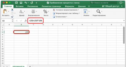
Let's look at a specific example. We need to add 10% of the same number to the number 250. To do this, we write the following expression in the cell / formula bar: “ =250+250*10% “.

After that, press “Enter” and get the finished result in the selected cell.

Earlier we already figured out how to do the calculations manually. Now let's look at how to perform calculations with data already entered in the table.

Adding a Percentage to an Entire Column

There are cases when we have an even more filled table, in which, along with the initial values in one column, there is also data with percentages in another, and the percentage values \u200b\u200bcan be different from each other.

In Excel, you can perform the most complex calculations with various units of data, whether it be finance, time, or ordinary numbers. Each case has its own nuances, and then we will focus on how to add numbers, dates (day, month, year) and percentages in Excel.

How to add numbers in Excel?

You can add numbers in Excel by writing a formula for adding two cells with data, or you can write the numbers themselves in the formula right away or add a number to a cell. The way to write a formula that uses cell addresses with values is more universal, since later it can be applied to other data and not rewritten when changing values, which can simply be written in the corresponding cell.

How to add date in Excel?

The easiest way to add a date in Excel is to add a value corresponding to the number of days to be added to the date written in the cell.

To make this whole process more understandable, you need to have an idea of how the date value is stored in Excel. And the date in Excel is stored as a numeric value corresponding to the number of days from January 1, 1900 up to the date value specified in the cell. That is, if you write a number in a cell "one" and assign the date format to the cell, then the cell will display the value 1.01.1900 .

Knowing this nuance, it is very easy to make a formula and add any number of days to the date in the cell.

It is much more difficult in Excel to add a month or a year to a specified date, but to simplify this process, there is a function THE DATE(). The function syntax is as follows: DATE(year, month, day). Thus, adding several months or years to the date, you don’t have to think about the number of days in a particular month or year, since everything will be calculated automatically.

Let's try using this function in Excel to add five years, six months and thirty-one days to our date. In this case, the format of the cell with the result will be automatically converted to the date format.

How to add percentages in Excel?

You can add percentages to a number in Excel using the classic formula for calculating interest, you just need to correctly write down the corresponding formula.

A simple but very common task that can be encountered in everyday work. How to add percentages in Excel using a formula?

Let's look at a simple example again and look at this problem in detail. Let's say we have a table with the price of goods to which we need to add 18% VAT.

If you write the formula in cell "C2"

B2 + 18%, then such a formula will be incorrect, since we need to add not just 18%, but 18% of the initial price. Therefore, to the initial price of 320 rubles, we need to add another 18% of 320 rubles, that is, 320 * 0.18 = 57.6 or B2 * 0.18

So the final formula will look like this

=B2+B2*0.18 or =B2+B2*18%

Note! If you initially added percentages incorrectly, that is, by simply writing B2 + 18%, then this cell will automatically receive the percentage format, that is, it will automatically be multiplied by 100 and the% sign will be added. If this happened, then in the end, when you write the correct formula, you can get this result

To display the correct result, you need to change the cell format from percent to numeric. Select all the cells with the price including VAT, click on the right mouse button and select "Cell Format", in the window that opens, select "Numeric" and click on "OK"

A simple task, but many people ask similar requests, so we decided to cover it as a separate article and describe it in such a way that it is clear why this is so.

I hope that the article helped you in solving your problem. We will be grateful if you click on the social buttons +1 and "Like" below this article.

During calculations, sometimes you need to add percentages to a specific number. For example, to find out the current profit indicators, which have increased by a certain percentage compared to the previous month, you need to add this percentage to the previous month's profit. There are many other examples where you need to perform a similar action. Let's see how to add a percentage to a number in Microsoft Excel.

Computational actions in a cell

So, if you just need to find out what the number will be equal to after adding a certain percentage to it, then you should enter the expression according to the following template into any cell of the sheet, or into the formula bar: “= (number) + (number) * (percent_value )%".

Let's say we need to calculate what number we get if we add twenty percent to 140. We write the following formula in any cell, or in the formula bar: "=140+140*20%".

Applying a Formula to Table Actions

Now, let's figure out how to add a certain percentage to the data that is already in the table.

First of all, select the cell where the result will be displayed. We put the sign "=" in it. Next, click on the cell containing the data to which the percentage should be added. We put a "+" sign. Again, click on the cell containing the number, put the "*" sign. Next, type on the keyboard the percentage by which you want to increase the number. Do not forget to put the sign "%" after entering this value.

Click on the ENTER button on the keyboard, after which the result of the calculation will be displayed.

If you want to extend this formula to all column values in the table, then simply stand on the lower right edge of the cell where the result is displayed. The cursor should turn into a cross. We press the left mouse button, and with the button held down, “stretch” the formula down to the very end of the table.

As you can see, the result of multiplying numbers by a certain percentage is also displayed for other cells in the column.

We found out that adding a percentage to a number in Microsoft Excel is not that difficult. However, many users do not know how to do this and make mistakes. For example, the most common mistake is writing a formula using the algorithm "=(number)+(percentage_value)%", instead of "=(number)+(number)*(percentage_value)%". This guide should help you avoid such mistakes.

We are glad we were able to help you resolve the issue.

Ask your question in the comments, describing in detail the essence of the problem. Our experts will try to answer as quickly as possible.

Did this article help you?

In various activities, the ability to calculate percentages is necessary. Understand how they "get". Trading allowances, VAT, discounts, returns on deposits, securities, and even tips are all calculated as some part of the whole.

Let's understand how to work with percentages in Excel. A program that performs calculations automatically and allows variations of the same formula.

Working with percentages in Excel

Calculating a percentage of a number, adding, subtracting interest on a modern calculator is not difficult. The main condition is that the corresponding icon (%) must be on the keyboard. And then - a matter of technique and attentiveness.

For example, 25 + 5%. To find the value of an expression, you need to type a given sequence of numbers and signs on the calculator. The result is 26.25. You don't need to be smart with this technique.

To create formulas in Excel, let's remember the school basics:

A percentage is a hundredth of a whole.

To find the percentage of a whole number, you need to divide the desired share by the whole number and multiply the total by 100.

Example. Brought 30 units of goods. On the first day, 5 units were sold. What percentage of the product was sold?

5 is a part. 30 is an integer. We substitute the data in the formula:

(5/30) * 100 = 16,7%

To add a percentage to a number in Excel (25 + 5%), you must first find 5% of 25. At school, they made up the proportion:

X \u003d (25 * 5) / 100 \u003d 1.25

After that, you can perform addition.

When basic computing skills are restored, it will not be difficult to figure out the formulas.

How to calculate percentage of a number in Excel

There are several ways.

We adapt the mathematical formula to the program: (part / whole) * 100.

Look carefully at the formula bar and the result. The result is correct. But we didn't multiply by 100. Why?

Cell format changes in Excel. For C1, we assigned the "Percentage" format. It involves multiplying the value by 100 and displaying it with a % sign. If necessary, you can set a certain number of digits after the decimal point.

Now let's calculate how much it will be 5% of 25. To do this, enter the calculation formula into the cell: \u003d (25 * 5) / 100. Result:

Or: =(25/100)*5. The result will be the same.

Let's solve the example in a different way, using the % sign on the keyboard:

Let's apply the acquired knowledge in practice.

The cost of the goods and the VAT rate (18%) are known. You need to calculate the amount of VAT.

Multiply the cost of the item by 18%. Let's "multiply" the formula to the entire column. To do this, click on the bottom right corner of the cell and drag it down.

The amount of VAT, the rate is known. Let's find the cost of the goods.

Calculation formula: =(B1*100)/18. Result:

The quantity of goods sold, individually and in total, is known. It is necessary to find the share of sales for each unit relative to the total.

The calculation formula remains the same: part / integer * 100. Only in this example, we will make the reference to the cell in the denominator of the fraction absolute. Use the $ sign before the row name and column name: $B$7.

How to add a percentage to a number

The problem is solved in two steps:

Find the percentage of a number. Here we have calculated how much will be 5% of 25.
Let's add the result to the number. Example for reference: 25 + 5%.

And here we have performed the actual addition. We omit the intermediate action. Initial data:

The VAT rate is 18%. We need to find the amount of VAT and add it to the price of the goods. Formula: price + (price * 18%).

Don't forget the brackets! With their help, we establish the order of calculation.

To subtract a percentage from a number in Excel, follow the same procedure. Only instead of addition, we perform subtraction.

How to calculate percentage difference in Excel?

How much the value has changed between two values as a percentage.

Let's abstract from Excel first. A month ago, tables were brought to the store at a price of 100 rubles per unit. Today the purchase price is 150 rubles.

Percent difference = (new data - old data) / old data * 100%.

In our example, the purchase price of a unit of goods increased by 50%.

Let's calculate the percentage difference between the data in the two columns:

Do not forget to set the "Percentage" cell format.

Calculate the percentage change between rows:

The formula is: (next value - previous value) / previous value.

With this arrangement of data, we skip the first line!

If you need to compare data for all months with January, for example, use an absolute cell reference with the desired value ($ sign).

How to make a percentage chart

First option: make a column in the data table. Then use this data to build a chart. Select the cells with percentages and copy - click "Insert" - select the chart type - OK.

The second option is to format the data labels as a share. In May - 22 working shifts. You need to calculate in percentage: how much each worker worked. We compile a table where the first column is the number of working days, the second is the number of days off.

Let's make a pie chart. Select the data in two columns - copy - "Insert" - chart - type - OK. Then we insert the data. Click on them with the right mouse button - "Format Data Signatures".

Select "Shares". On the "Number" tab - percentage format. It turns out like this:

Download all examples with percentages in Excel

We will stop there. And you can edit to your taste: change the color, the appearance of the diagram, make underlines, etc.

A simple but very common task that can be encountered in everyday work. How to add percentages in Excel using a formula?

Video: How to quickly calculate percentages in Excel 2007

Let's look at a simple example again and look at this problem in detail. Let's say we have a table with the price of goods to which we need to add 18% VAT.

If you write the formula in cell "C2"

So the final formula will look like this

B2+B2*0.18 or =B2+B2*18%

Video: How to calculate percentages in Excel?

A simple task, but many people ask similar requests, so we decided to cover it as a separate article and describe it in such a way that it is clear why this is so.

I hope that the article helped you in solving your problem. We will be grateful if you click on the social buttons +1 and "Like" below this article.

The Microsoft Office Document Creation Suite is a popular suite of programs. Every person who typed information on a computer, compiled lists, calculated various indicators, and created presentations to demonstrate them to an audience is familiar with them. Among the programs of the package, Excel deserves special attention - an assistant in carrying out various calculations. To determine% of a number, adding percentage values, it is worth knowing some of the nuances that will simplify the calculations.

Cell Format

Before entering a formula in a cell, you should set the format to "percentage". In this case, there is no need to enter additional steps. A “%” icon will automatically be placed next to the received value.

Basic Formula

In Excel, there are general rules for calculating interest. After selecting the cell format, enter the formula.

The basic formula for interest in Excel is written as follows:

The "=" sign is placed.

The cursor presses the value whose percentage is to be calculated.

An oblique dividing line is set from the keyboard.

Then the cell to which the percentage is calculated is pressed.

Calculation of percentages in Excel in a column

Sometimes it is necessary to calculate the percentages of values that are located in columns. To do this, you need to enter the basic percentage formula in Excel in the first cell of the column, then, by clicking in the lower right corner of the cell, “drag” down to calculate the desired values.

Calculating Percentages in Rows

When data is written horizontally, in rows, interest is calculated in the same way as in columns. After selecting the cell format, the percentage formula is entered into the Excel spreadsheet.

The “equal” icon is put, the cell is selected, the percentage of which needs to be calculated. Then - the line of division. The value of the cell to which you want to calculate the percentage is selected.

After that, you need to click on the lower right corner of the cell with the cursor and drag it to the side until the required values are calculated.

Calculation from the total amount

To do this, you can put the "=" sign and, highlighting the cells one by one, press the "+" sign between them. Then the Enter key is pressed.

You can also, after putting down “=”, type SUM on the keyboard, open the bracket, enter the range of cells for summation, and then press Enter.

When calculating the share of the total amount, after the introduction of the “equal” sign, in the cells whose share needs to be calculated, the “$” signs are placed in front of the row number and the column letter. This icon "fixes" the relationship between them. Without this sign, interest will be calculated from other cells.

Adding percentages to a number

Before you add percentages to a number in Excel, you should familiarize yourself with the general calculation formula. Do not forget that a percentage is a hundredth of a number.

If you need to add Excel percentages to a column of values, you can enter the following formula: "=" icon, the cell to which you want to add percentages, the percentage value, the "/" sign, the same cell to which percentages are added multiplied by one hundred.

If the percentage value is placed in a separate column or cell, the formula will look different.

Before you add a percentage to a number in another column in Excel, the formula must take the form: equals sign, cell to which you want to add percentages, plus sign, cell with the percentage value with "$" signs, multiplied by the cell to which we add percentages. Provided that the latter format is set to "percentage".

If percentages are in one column, and the values to which you want to add them are in another, then the formula that allows Excel to add percentages to a number will take the following form: equals sign, cell with value, plus sign, cell with percent, multiplied by the cell with the number. It is important not to confuse cell formats! Percentage format can only be set for cells with %.

When calculating % in Excel, remember to set the cell format for percentage values. For cells with numbers, a numeric value is used, for percentages, a percentage value. You can select it from the menu that appears after pressing the right mouse button.

In all formulas for calculating interest, the “=” sign is required. If you do not put it, the formula will not calculate.

Calculations in columns and rows are similar. Many operations are performed by "stretching" cells. To do this, enter the calculation formula and click on the cross in the lower right corner of the cell. Then use the cursor to "stretch" the value down, up or in the desired direction. The calculation will happen automatically.

There are several formulas that allow you to add percentages to a number in Excel. It depends on whether you need to add a specific value or data from another column.

If you need to add percentages of one cell, calculate a fraction of one value, use the "$" sign, which is installed in the formula bar before the line number and column letter.